Table of Contents
Slow Speed Considerations
Some users find it necessary to run stages at very slow and steady scanning speeds. For a mechanical stage system, ASI stages and controllers manage to do a pretty good job of this, but there are limitations. This document helps to clarify what has been observed at very slow speeds and what can be expected of the stage in various configurations.
Controller Limitations
The WK controller has 16-bit dynamic velocity range available. The controller operates internally with distances in encoder counts and time steps in servo cycles (Tstep). The natural minimum speed is one encoder count per servo cycle. In many instances, this natural minimum speed is still too fast, so velocity scaling is included in the controller. The table below shows the dynamic control range available for various typical system configurations.
| Encoder Resolution(nm) | Encoder Type | Lead-screw pitch(mm) | Num of Axes | Servo Tstep (ms) | Velocity SCALE factor | Controller Dynamic Range | Max Stage Speed(with standard motors) (mm/sec) | |
|---|---|---|---|---|---|---|---|---|
| Min Speed (µm/s) | Max Speed (mm/s) | |||||||
| 2.2 | Rotary | 0.635 | 3 | 0.75 | 64 | 0.046 | 1.5 | 0.7 |
| 5.5 | Rotary | 1.59 | 3 | 0.75 | 64 | 0.114 | 3.8 | 1.75 |
| 5.5 | Rotary | 1.59 | 2 | 0.5 | 64 | 0.171 | 5.6 | 1.75 |
| 5.5 | Rotary | 1.59 | 1 | 0.5 | 64 | 0.171 | 2.8 | 1.75 |
| 22 | Rotary | 6.35 | 3 | 0.75 | 64 | 0.458 | 15.0 | 7 |
| 22 | Rotary | 6.35 | 1 | 0.5 | 64 | 0.688 | 11.3 | 7 |
| 44 | Rotary | 12.7 | 3 | 0.75 | 64 | 0.917 | 30.0 | 14 |
| 10 | Linear | n/a | 3 | 0.75 | 64 | 0.208 | 6.8 | n/a |
| 20 | Linear | n/a | 2 | 0.5 | 64 | 0.625 | 20.5 | n/a |
The chart above shows the controller’s maximum controlled speed as well as the maximum speed obtainable for a particular leadscrew. The actual minimum speeds obtainable will also have something to do with the motor-controller-bearing dynamics. It is this issue that we examine next by looking at actual low speed motion histories.
Optical Tracking Tests
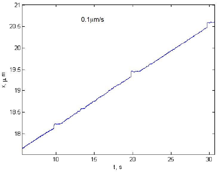
The next three plots show actual stage motion as determined by looking at the position of an object optically and plotting its location. The first plot shows a stage with 1.59 mm pitch lead screws and rotary encoders traveling at its slowest controlled speed, about 0.1 μm/sec. There are distinct glitches in the motion every 10 seconds or so, corresponding to motion of about 1.25 μm.
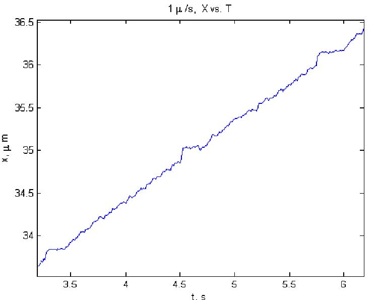
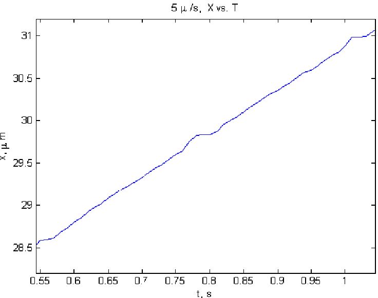
The second and third plots show motion where the stage was commanded to go about 1 μm/sec and 5 μm/sec respectively. Both plots also show the glitches, still about 1.25 μm apart, now occurring more frequently because of the faster speeds. Hence, it appears that the glitches are due to some fixed mechanical disturbance to the system.
The movement per motor turn can be calculated as follows:
\begin{equation} D = \frac{screw-pitch}{gearhead-reduction} \\ D = \frac{1.59}{141} = 11.3 μm/rev \end{equation}
With the spacing of the glitches at 1.25 μm, we are seeing about 9 glitches per turn. This turns out to be exactly the number of teeth on the primary motor gear in the anti-backlash gearhead on the motor. The anti-backlash gearhead consists of two identical parallel gear trains, locked in preloaded torsional opposition at the motor and output shaft. Perhaps the output shaft jumps ahead as a gear tooth is released and then abruptly halts as the next tooth catches it. At the very slowest speed, the servo loop has plenty of time to ensure that the motor is turning quite uniformly, even in the presence of torque variations caused by the glitches. Indeed, data taken from the motor encoders show very short glitches of 5-6 encoder counts, whereas the displacements seen in the optical measurements would be closer to 20-30 encoder counts lasting much longer – consistent with this explanation. It is clear that regulating strongly on the rotary encoder so that the motor will turn at a uniform rate will not significantly reduce the speed variations in the output shaft. It would be more effective to regulate on stage linear encoders and attempt to modify the motor speed to compensate for the glitches. Because of their sudden time varying nature, this approach will only yield marginal improvement, especially at intermediate speeds between 1 μm/s and 20 μm/s. Experiments would need to be done to see if aggressive servo loop tuning could improve the response enough to make a significant difference using the linear encoders.
Scanning Experiments
The problems of uneven slow-speed operation reared its head again during slow speed scanning experiments using the controller’s SCAN mode functions. Again the problem was traced to the periodic variations in speed caused by the motor gear teeth on the anti-backlash gearhead. The problems were reported in both rotary and linear encoder mode. Since the anti-backlash gear preload is suspected to be the origin of the uneven movement, several experiments were done using bare motors, i.e., motors not installed in stages. SCAN firmware was used to initiate several low-speed scans, and the encoder divide-by-N signal pulses were recorded on an oscilloscope. Data was taken first using a standard off-the-shelf stage motor, then with a motor where the preload on the anti-backlash gear had been removed by pulling the gearhead and replacing it with no torsion on its gear trains. Typical data recordings for the two motor configurations are shown below.
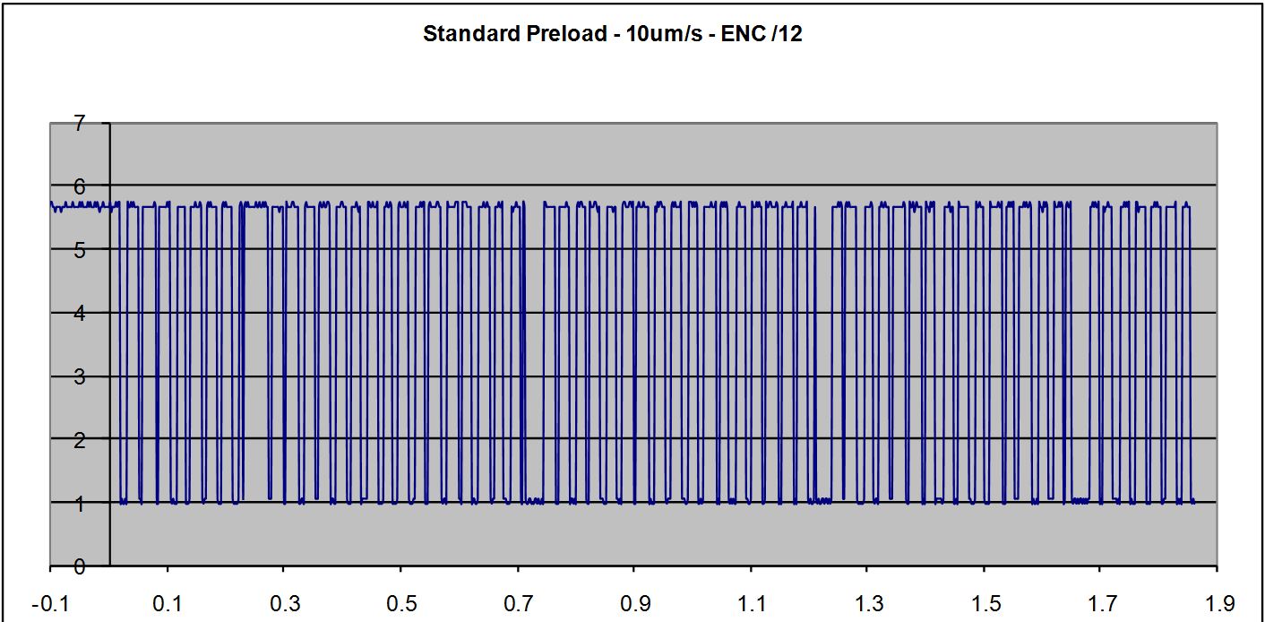
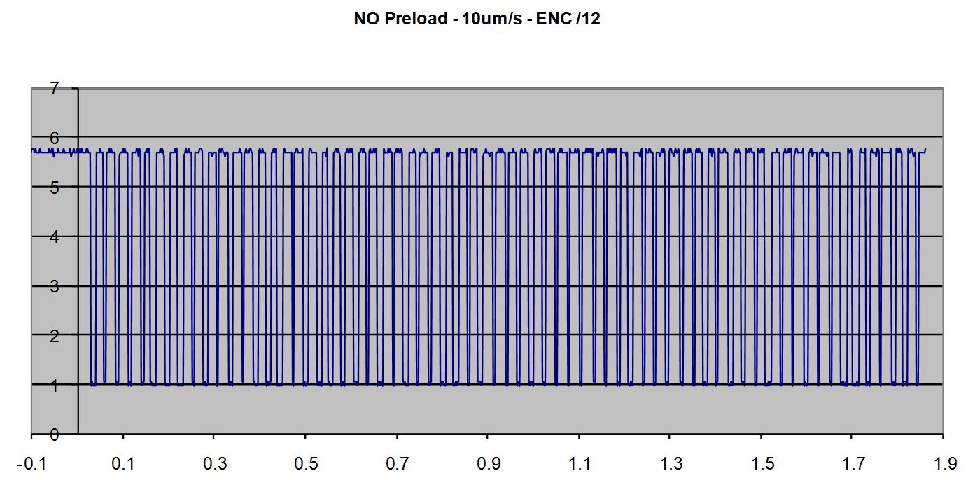
Removing the anti-backlash preload significantly smoothes out the motion. The table below summarizes the results of several runs using various scanning speeds and encoder counts per output pulse. The average pulse separation time, ⍑, and the standard deviation of the time, σ, as well as the maximum variation, TVAR, defined as:
\begin{equation} T_{VAR}≡[{[ \frac{MAX(Δt)}{⍑}+ \frac{⍑}{MIN(Δt)}]\over 2} – 1 ] × 100 \end{equation}
are shown in the table below. Perfect uniformity would have TVAR = 0%; TVAR = 100% would mean that the spacing would be shifting by amounts about the same order as the average spacing.
| 1.59 mm Pitch | 6.35 mm Pitch | Encoder Counts per pulse | Standard Gearhead with Preload | NO Preload | ||||||
|---|---|---|---|---|---|---|---|---|---|---|
| Speed (μm/s) | Δx(nm) | Speed(μm/s) | Δx(nm) | ⍑(ms) | σ(ms) | TVAR % | ⍑(ms) | σ(ms) | TVAR % | |
| 1 | 198 | 4 | 792 | 36 | 221 | 59 | 63 | 216 | 8.5 | 9.5 |
| 2.5 | 66 | 10 | 264 | 12 | 27.3 | 6.7 | 165 | 27.5 | 3.3 | 12 |
| 10 | 198 | 40 | 792 | 36 | 19.7 | 1.6 | 19 1 | 9.3 | 3.4 | 11 |
| 10 | 66 | 40 | 264 | 12 | 6.72 | 1.8 | 108 | 6.62 | 0.85 | 30 |
| 100 | 66 | 400 | 264 | 12 | 0.66 | 0.05 | 21 | 0.66 | 0.04 | 12 |
The trends that emerge confirm expectations that the problem is greatest at slow speeds, and that averaging the motion over more encoder counts reduces the apparent speed variation. It also shows that removing the preload makes a dramatic difference in speed uniformity.
For those wishing to obtain smooth slow-speed motion – the recommendations would be to 1) use fine pitch lead screws so the motor speed can be as fast as possible, 2) use linear encoders so that the speed variation at the stage becomes visible to the control loop and can be reduced by the servo system, and 3), for critical systems, use motors without the anti-backlash gear preload.
As of 2015 ASI routinely offers “scan-optimized” stages that do not have the anti-backlash gearing in the scan axis (usually X) and almost always have 16 TPI (1.59mm pitch) leadscrews. These are recommended for smoothest scanning.
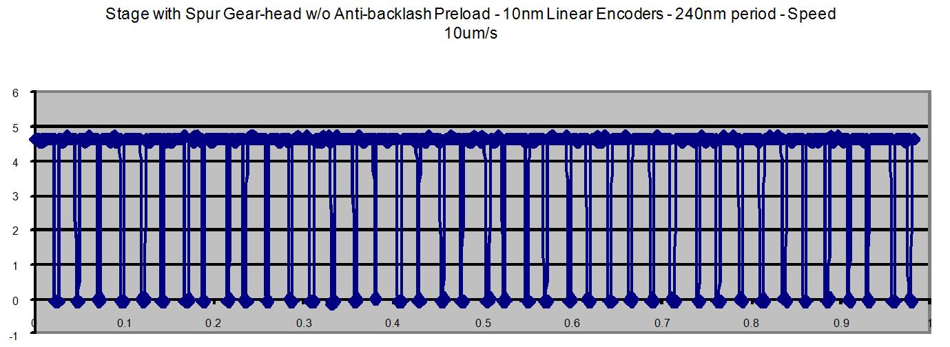
Tests on Stage with Linear Encoder and Spur Gearhead
Based upon the above considerations, a stage equipped with linear encoders and a standard spur gearhead motor without the zero-backlash feature was set up and tested. A representative typical scan is shown below for the stage traveling at 10 μm/sec with encoder pulses every 240 nm. This stage was equipped with 1.59 mm pitch lead screws. None of the very obvious speed fluctuations seen with the zero-backlash gearhead are present. The speed is still not perfectly uniform, undoubtedly because of small mechanical imperfections in the motor and bearing systems.
Quantitative measurements of the velocity uniformity were made for various commanded scanning speeds. The results of the tests are summarized below.
| Stage with 1.59 mm pitch lead screw, 10 nm linear encoders | Encoder ÷ 24 Δx = 240 nm | Encoder÷12 Δx = 120 nm |
|||||
|---|---|---|---|---|---|---|---|
| Nominal Speed (μ/s) | Ideal Realized Speed (μ/s) | ⊽ (μ/s) | σ (μ/s) | VVAR % | ⊽ (μ/s) | σ (μ/s) | VVAR % |
| 1 | 0.92 | 0.84 | 0.10 | 49 | |||
| 2 | 1.95 | 1.87 | 0.24 | 41 | |||
| 5 | 4.93 | 5.02 | 0.45 | 25 | 5.02 | 0.98 | 69 |
| 10 | 9.98 | 10.09 | 1.2 | 29 | |||
| 20 | 19.96 | 20.08 | 2.9 | 35 | |||
\begin{equation} V_{VAR}≡[{[ \frac{MAX(V)}{⊽}+ \frac{⊽}{MIN(V)}]\over 2} – 1 ] × 100 \end{equation}
The instantaneous velocity, V, is calculated as Δx/Δt for each output signal pulse edge. The MAX(V) and MAX(V) values are determined from the MIN(Δt), and MAX(Δt), found during the full scan, respectively.
Conclusions
Data for the 5 μm/s runs was collected for both 120 nm and 240 nm sampling intervals. Clearly, the averaging effect of the larger sampling interval reduces the measured speed variation, as one would expect.
The results show tolerably uniform velocities at very slow scanning speeds when the velocity is determined over a distance < 0.25 μm. Users that require this level of performance should contact ASI to determine the most appropriate motor / lead screw combination for the application.