Table of Contents
Epi-Illumination Options and Laser Coupling
The flexibility of the light path on the ASI Modular Infinity Microscope (MIM) brings with it the challenge of properly designing epi-illumination so that the desired intensity and uniformity of the illumination light are achieved. We will discuss various fluorescence illumination condenser options and the pros and cons of various approaches.
Critical Illumination
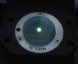
Critical illumination focuses the light source into the sample plane. This is an efficient and simple method of illumination, but any non uniformity in the light source will appear at the sample, so this method is restricted for use with a very uniform source. One such source is the output of a liquid light guide illuminator. Multiple internal reflections in the light guide produce a fairly uniform illumination intensity across the end of the light guide. A simple arrangement for critical illumination is shown in the figure below.

The field size of the illumination is determined by the diameter of the light guide tip, and the relative focal lengths of the light-guide condenser lens and the objective. Since the objective lens will vary, it is better to compare with the field at the camera image plane, determined by the tube lens focal length. At the camera, the size of the illumination image can be calculated for a typical example.
\begin{equation} FOV=d_{Light Guide} \frac{F_{Tube Lens}}{F_{Condenser}} =3mm \frac{200 mm}{25 mm}=24mm \end{equation}
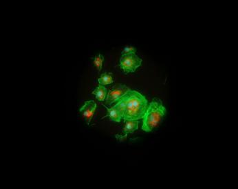
Here is an image of a fluorescent test sample made with critical illumination using the C60-LLG_ADPT as the condenser. The Sony APC camera sensor is 23.4 x 15.6 mm (28mm diagonal) so it is not surprising that you can see the edges of the illumination defined by the projected image of the end of the light guide itself.

It becomes more problematic to use critical illumination with a light source that has some structure, such as a lamp filament or and LED. The next photo shows what happens if you use an LED illuminator in this mode of illumination. You can clearly see the structure of the LED die imposed in the image.

Another drawback to this simple arrangement is that there is no place to include a field stop, so regions outside the camera sensor area will unnecessarily be exposed to light. Because the light beam from the collector lens to the objective aperture is roughly collimated, there is quite a bit of flexibility in how far the illuminator can be from the objective lens. The iris on the liquid light guide adapter will act as an aperture control. However, the light incident on the objective back focal plane is a broad beam and will expand with distance. Objectives with a small aperture will not optimally make use of the available light, and much of the light will be lost inside the microscope tubes. The photos to the right shows what happens as you open the aperture on the light source (here an LED illuminator was used). Flooding the inside of the the objective tube with unused light is never a good idea.


Both of these limitations can be eliminated with a more elaborate condenser arrangement that includes a couple more lenses as shown in the figure below.

Here a pair of 100mm tube lenses makes are relay optic where the lenses are arranged with iris diaphragms to provide both a field stop (iris co-focal with the sample) and an aperture stop (iris focused at objective back focal plane). Figures 6 and 7 shown illustrate the effects of the two stops. This condenser is still operating with critical illumination, so the tip of the light guide is still focused into the sample plane. Hence the apparent size of the light guide remains the maximum limit to the field of view of the illumination.
One of the main advantages of this condenser is the ability to accurately stop the aperture so that light that cannot be used by the objective lens will be eliminated before it enters the beam splitter cube, where the stray light could be scattered into the imaging path. The size of the objective pupil can vary from just a couple of millimeters for high-magnification, low-NA objectives to more than 15mm for high-NA low-magnification objectives.
The ASI C60 MIM components allow the relatively complex optical assemblies to be simply constructed. Using standard C60-TUBE_xxx lenses and the C60-LAMP-ADPT, the iris in components that are attached to the C60-LAMP_ADPT will be at the focus of the lenses. C60_EXT_xx extension tubes can be used to make up the correct distance to the back focal point of the tube lenses. Perfect focus at the back focal point is usually not critical, and is often not possible to know exactly unless at fixed focus position and specific objective lens is specified.
Kohler Illumination
With Kohler illumination the light source is imaged to the back focal plane of the objective lens. This ensures that structure in the light source does not appear in the image. In our configuration the iris diaphragm of the collector lens is imaged at the specimen plane and thus provides a field stop. A Kohler condenser can be constructed from a tube lens and the C60-LAMP_ADPT, which functions as the appropriate spacer to focus the tube lens at the iris in the illuminator. A diagram of the condenser is shown in Figure 8 below.

There are two constraints that must both be satisfied to get optimum results.
- Collimated light from the illuminator needs to be refocused at approximately the objective lens back focal plane. This constraint is generally not met exactly unless care is taken, but ASI's LED sources can be easily adjusted in the field to meet this condition.
- The illuminator iris must be at the focal point of the tube lens. This is guaranteed by the construction conventions of the ASI tube lenses and the length of the
C60-LAMP_ADPT.
Focusing to objective back focal plane
Alignment and proper focusing of the light source can best be accomplished using a witness target at roughly the back focal plane of the objective lens. In most cases, the location of the objective back focal plane is not at the flange of the objective. Assuming that the back focal distance of the condenser tube lens comes close to focusing at the objective back focal position, you should be able to get a good focus on the witness target by adjusting the axial position of the light source (loosening the light guide set-screw or rotating the LED housing of the LED Lamp along its helical threads). Center the focused spot / image of the LED die in the aperture. Use the kinematic adjusters on the C60-CUBE-III dichroic cube to adjust centering if necessary.

The image above shows very good illumination into the corners of the full field of the camera. The tip of the light guide was focused to the objective back focal plane as shown in the figure below. The image size of the light guide tip at the back focal plane will be magnified by the ratio of the focal lengths of the tube lens and collector lens, in this case 100/25. Hence the image of the light guide tip will be about 3 mm x 100/25 = 12 mm. The 20X NA 0.75 objective, used to make the images above, has a back aperture diameter of 15mm so all of this light will enter the objective pupil. Lower numerical aperture or higher magnification objectives will have a smaller pupil, so light can still be lost. One can see the reason for a smaller diameter light guide when optimally coupling to higher magnification objectives. For instance, a 1.5mm diameter light guide would be magnified to 6mm which is near the pupil size of oil immersion 40X and 60X objectives, so there would be still be good coupling efficiency.

Kohler illumination is even more important with non-uniform light sources such as filaments or LEDs. The image below was taken using a high intensity white LED as the light source. The image of the LED die is shown in Figure 12. Despite the distinct structure of the die, the image illumination is uniform with the Kohler arrangement.

The image size of the field stop translates into the image field of view. The ratio of the camera tube lens focal length compared to the condenser tube lens will determine the field size for a given aperture. In our example this is 200mm / 100mm, so the camera field of view is twice the aperture size. This might seem a waste, because the collector lens is a full 25 mm in diameter, so we must be wasting some light. Furthermore, if the distribution of the light from the source is not uniform, what ensures a uniform fill at the field stop – which is reflected in the image? These issues are best addressed by considering the angular distribution of the light coming from various light sources.

Rule of thumb: If you are filling both the objective pupil and the field aperture you cannot do any better.
Liquid Light Guides
Optical light guides are very popular as the effective sources for microscope illumination. They provide a simple and flexible way to bring light from a possibly hot source to the microscope platform. The main characteristic of light guides is the critical angle that defines the acceptance angle and numerical aperture of the guide. Light outside the acceptance cone cannot propagate in the light guide and will be lost. The main disadvantage of a light guide is that the intrinsic brightness of an arc source will be diminished because of the larger diameter of the light guide core. In any optical system the intrinsic brightness, defined by the reciprocal of the numerical aperture (divergence of the light) and the diameter of the source is a canonical constant and can only diminish as light propagates through an optical system. This concept can be expressed as the Lagrange invariant for refractive index n, ray radius r, and ray angle θ.
\begin{equation} n_1r_1θ_1=n_2r_2θ_2 → NA d≅ \frac{n d^2}{2 f.l.} = constant \end{equation}
We can use this concept to identify how best to utilize the light available to us. Note this is closely related to the concept of etendue.
Table 1: Relative brightness and Lagrange invariant for various Light Sources
| \begin{equation}NA d \end{equation}(mm) | Light Source | Relative intrinsic Brightness \begin{equation} \frac{1}{NA d} \end{equation} | Power Density for 100 mW source \begin{equation} \frac{W}{mm^2} \end{equation} |
|---|---|---|---|
| 1.93 | LED with 3mm dia. Emitter, +/-40⁰ pattern. | 0.52 | 0.014 |
| 1.5 | 3mm NA 0.5 Light guide | 0.67 | 0.014 |
| 0.5 | 1mm Arc w/ F1 Lens | 2.0 | 0.4 |
| 0.33 | 1.5mm NA 0.22 Light Guide | 3.0 | 0.056 |
| 0.011 | Multi-mode fiber; 0.050, NA 0.22 | 91 | 51 |
| 0.0004 | Single mode fiber; 0.004mm, NA 0.1 | 2500 | 7958 |
Table 2: Lagrange Invariant NA d for objectives and tube lenses
| \begin{equation}NA d \end{equation} (mm) | Optical component (assume 25mm camera FOV) | Maximum possible coupling efficiency from 3mm NA 0.5 LG | Objective back pupil size (mm) |
|---|---|---|---|
| 1.98 | 100mm F.L. 33mm dia. Tube Lens w/ 12mm image | 100% | |
| 1.98 | 160mm F.L. 33mm dia. Tube Lens w/ 19.2mm image | 100% | |
| 1.75 | Objective: 4X NA 0.28 | 100% | 28.0 |
| 1.13 | Objective: 10X NA 0.45 | 56% | 18.0 |
| 0.94 | Objective: 20X NA 0.75 | 39% | 15.0 |
| 0.58 | Objective: 60X NA 1.4 | 15% | 6.14 |
| 0.35 | Objective: 100X NA 1.4 | 5.4% | 3.68 |
The tables above illustrate the advantage of using a bright source if you wish to couple light efficiently into a high magnification objective. Only about 5% of the light from a 3mm liquid light guide can be coupled into the 100X, NA 1.4 objective, however, all of the light from a 1.5mm NA 0.22 light guide, or fiber optic light source could be used.
Laser Illumination
Laser Epi-Illumination
Lasers are very bright sources, which makes them easy to couple efficiently into the microscope. However a Gaussian single mode laser beam does not have a uniform intensity distribution, so the illumination profile will not be uniform. The simplest way to get a moderately uniform illumination profile is to over-expand the beam so that only the central section is used for illuminating the field of view. However, this approach wastes laser power as illustrated in the table below.
Table 3: Truncated Gaussian Beam Illumination
| Apertured Gaussian \begin{equation} \frac{r}{w} \end{equation} | Intensity Uniformity \begin{equation} \frac{I(r)}{I_0} \end{equation} | Laser Power Efficiency \begin{equation} \frac{P(r)}{P_0}\end{equation} (%) |
|---|---|---|
| 0.1 | 0.98 | 2.0 |
| 0.2 | 0.923 | 7.7 |
| 0.4 | 0.726 | 27.4 |
| 0.7 | 0.375 | 62.5 |
| 1.0 | 0.135 | 86.5 |
Nevertheless, this is a simple way to illuminate a sample with a laser. A condenser built with standard modular microscope components is illustrated in Figure 13. The second tube lens should be chosen to focus approximately in the objective back focal plane, as usual. The first tube lens can be selected to either capture all of the light from the fiber into the camera illumination field of view, or it can be deliberately chosen with a longer focal length so that only the central section of the laser spot, which is more uniform, will pass the field stop.

The light field diameter for various collection tube lenses is shown in Table 4 below. The relative size of the light field at the camera will depend upon the ratio of camera tube lens to the condenser tube lens. For instance, from Table 4, using a 160 f.l. collector lens and an 11.5mm field stop, the uniformity of the light field would be 73%. If the condenser tube lens was 100mm and the camera tube lens was 200mm, then the fluorescence illumination would fill a 23mm diameter field at the camera.
Laser Spot Illumination
If you wish to project a focused laser spot into the sample plane, you can use the condenser about but without the second tube lens, Figure 14.

In this case the iris diaphragm can be used as an aperture intensity control. It will also inversely determine the minimum focused beam waist at the sample. For apertures larger than the objective pupil, the laser illumination will be lost entering the objective. Smaller collimated beam diameters can be obtained using fiber collimators, such as ASI’s FCOL-PC12.5. Steering the beam accurately into the back focal plane can be accomplished with the adjustable mirror on the C60_BEAMSPLITTER-II.
Table 4: Light field diameter for various fibers, light guides, and collection optics.
| Light Field Diameter | ||||||
|---|---|---|---|---|---|---|
| SM Gaussian Power Fraction within aperture listed | 95% | 86.50% | 27.40% | |||
| Light Guide Numerical Aperture and Collector Lens | NA dia. | Gaussian Waist | Truncated Gaussian - 73% uniformity | |||
| Type of Lightguide | Fiber NA | Lens Focal Length (mm) | dNA (mm) | dGauss(mm) | dAperture(mm) | ASI Coupling Lens Component |
| Single Mode Fiber | 0.11 | 200 | 44 | 6.1 | 14.4 | C60_Tube_200 |
| Single Mode Fiber | 0.11 | 160 | 35.2 | 28.9 | 11.5 | C60_Tube_160 |
| Single Mode Fiber | 0.11 | 100 | 22 | 18.0 | 7.2 | C60_Tube_100 |
| Single Mode Fiber | 0.11 | 12.5 | 2.75 | 2.25 | FCOL-PC12.5 | |
| Multimode Fiber | 0.22 | 12.5 | 5.5 | FCOL-PC12.5 | ||
| MM Light Guide | 0.22 | 25 | 11 | MIM-LLG_ADPT | ||
| MM Light Guide | 0.22 | 100 | 44 | C60_Tube_100 | ||
| MM Light Guide | 0.5 | 25 | 25 | MIM-LLG_ADPT | ||
| MM Light Guide | 0.5 | 100 | 100 | C60_Tube_100 | ||